Exploratory Data Analysis Basics

EDA Definition

Razones para hacer un EDA

• Organizar y entender las variables

• Establecer relaciones entre las variables

• Encontrar patrones ocultos en los datos

• Ayuda a escoger el modelo correcto para la necesidad correcta

• Tomar decisiones informadas

Pasos de EDA

Tipos de Analitica de datos

Project

Environment Setup

Library installation

!pip install --upgrade pip

!pip install palmerpenguins==0.1.4 numpy==1.23.4 pandas==1.5.1 seaborn==0.12.1 matplotlib==3.6.0 empiricaldist==0.6.7 statsmodels==0.13.5 scikit-learn==1.1.2 pyjanitor==0.23.1 session-info

Requirement already satisfied: pip in c:\users\admin\miniconda3\envs\jupyter_notebooks_from_deepnote\lib\site-packages (23.2.1)

^C
Collecting palmerpenguins==0.1.4
  Using cached palmerpenguins-0.1.4-py3-none-any.whl (17 kB)
Collecting numpy==1.23.4
  Using cached numpy-1.23.4-cp311-cp311-win_amd64.whl (14.6 MB)
Collecting pandas==1.5.1
  Using cached pandas-1.5.1-cp311-cp311-win_amd64.whl (10.3 MB)
Collecting seaborn==0.12.1
  Using cached seaborn-0.12.1-py3-none-any.whl (288 kB)
Collecting matplotlib==3.6.0
  Using cached matplotlib-3.6.0-cp311-cp311-win_amd64.whl (7.2 MB)
Collecting empiricaldist==0.6.7
  Using cached empiricaldist-0.6.7.tar.gz (11 kB)
  Preparing metadata (setup.py): started
  Preparing metadata (setup.py): finished with status 'done'
Collecting statsmodels==0.13.5
  Using cached statsmodels-0.13.5-cp311-cp311-win_amd64.whl (9.0 MB)
Collecting scikit-learn==1.1.2
  Using cached scikit-learn-1.1.2.tar.gz (7.0 MB)
  Installing build dependencies: started

Library import

import empiricaldist
import janitor
import matplotlib.pyplot as plt
import numpy as np
import palmerpenguins
import pandas as pd
import scipy.stats
import seaborn as sns
import sklearn.metrics
import statsmodels.api as sm
import statsmodels.formula.api as smf
import statsmodels.stats as ss
import session_info

Stablish Chart Settings

%matplotlib inline
sns.set_style(style='whitegrid')
sns.set_context(context='notebook')
plt.rcParams['figure.figsize'] = (11, 9.4)

penguin_color = {
    'Adelie': '#ff6602ff',
    'Gentoo': '#0f7175ff',
    'Chinstrap': '#c65dc9ff'
}

Importing Dataset

The dataset chosen for this project is the palmerpenguins dataset

The goal of the Palmer Penguins dataset is to replace the highly overused Iris dataset for data exploration & visualization.

The information contains size measurements, clutch observations, and blood isotope ratios for 344 adult foraging Adélie, Chinstrap, and Gentoo penguins observed on islands in the Palmer Archipelago near Palmer Station, Antarctica.

Data were collected and made available by Dr. Kristen Gorman and the Palmer Station, Antarctica Long Term Ecological Research (LTER) Program.

Raw Data

This package contains a raw dataset (literally contains the data as it was collected)

raw_df = palmerpenguins.load_penguins_raw()

raw_df

	studyName	Sample Number	Species	Region	Island	Stage	Individual ID	Clutch Completion	Date Egg	Culmen Length (mm)	Culmen Depth (mm)	Flipper Length (mm)	Body Mass (g)	Sex	Delta 15 N (o/oo)	Delta 13 C (o/oo)	Comments
0	PAL0708	1	Adelie Penguin (Pygoscelis adeliae)	Anvers	Torgersen	Adult, 1 Egg Stage	N1A1	Yes	2007-11-11	39.1	18.7	181.0	3750.0	MALE	NaN	NaN	Not enough blood for isotopes.
1	PAL0708	2	Adelie Penguin (Pygoscelis adeliae)	Anvers	Torgersen	Adult, 1 Egg Stage	N1A2	Yes	2007-11-11	39.5	17.4	186.0	3800.0	FEMALE	8.94956	-24.69454	NaN
2	PAL0708	3	Adelie Penguin (Pygoscelis adeliae)	Anvers	Torgersen	Adult, 1 Egg Stage	N2A1	Yes	2007-11-16	40.3	18.0	195.0	3250.0	FEMALE	8.36821	-25.33302	NaN
3	PAL0708	4	Adelie Penguin (Pygoscelis adeliae)	Anvers	Torgersen	Adult, 1 Egg Stage	N2A2	Yes	2007-11-16	NaN	NaN	NaN	NaN	NaN	NaN	NaN	Adult not sampled.
4	PAL0708	5	Adelie Penguin (Pygoscelis adeliae)	Anvers	Torgersen	Adult, 1 Egg Stage	N3A1	Yes	2007-11-16	36.7	19.3	193.0	3450.0	FEMALE	8.76651	-25.32426	NaN
...	...	...	...	...	...	...	...	...	...	...	...	...	...	...	...	...	...
339	PAL0910	64	Chinstrap penguin (Pygoscelis antarctica)	Anvers	Dream	Adult, 1 Egg Stage	N98A2	Yes	2009-11-19	55.8	19.8	207.0	4000.0	MALE	9.70465	-24.53494	NaN
340	PAL0910	65	Chinstrap penguin (Pygoscelis antarctica)	Anvers	Dream	Adult, 1 Egg Stage	N99A1	No	2009-11-21	43.5	18.1	202.0	3400.0	FEMALE	9.37608	-24.40753	Nest never observed with full clutch.
341	PAL0910	66	Chinstrap penguin (Pygoscelis antarctica)	Anvers	Dream	Adult, 1 Egg Stage	N99A2	No	2009-11-21	49.6	18.2	193.0	3775.0	MALE	9.46180	-24.70615	Nest never observed with full clutch.
342	PAL0910	67	Chinstrap penguin (Pygoscelis antarctica)	Anvers	Dream	Adult, 1 Egg Stage	N100A1	Yes	2009-11-21	50.8	19.0	210.0	4100.0	MALE	9.98044	-24.68741	NaN
343	PAL0910	68	Chinstrap penguin (Pygoscelis antarctica)	Anvers	Dream	Adult, 1 Egg Stage	N100A2	Yes	2009-11-21	50.2	18.7	198.0	3775.0	FEMALE	9.39305	-24.25255	NaN

344 rows × 17 columns

processed data

Dataset containing already processed data

df = palmerpenguins.load_penguins()

df

	species	island	bill_length_mm	bill_depth_mm	flipper_length_mm	body_mass_g	sex	year
0	Adelie	Torgersen	39.1	18.7	181.0	3750.0	male	2007
1	Adelie	Torgersen	39.5	17.4	186.0	3800.0	female	2007
2	Adelie	Torgersen	40.3	18.0	195.0	3250.0	female	2007
3	Adelie	Torgersen	NaN	NaN	NaN	NaN	NaN	2007
4	Adelie	Torgersen	36.7	19.3	193.0	3450.0	female	2007
...	...	...	...	...	...	...	...	...
339	Chinstrap	Dream	55.8	19.8	207.0	4000.0	male	2009
340	Chinstrap	Dream	43.5	18.1	202.0	3400.0	female	2009
341	Chinstrap	Dream	49.6	18.2	193.0	3775.0	male	2009
342	Chinstrap	Dream	50.8	19.0	210.0	4100.0	male	2009
343	Chinstrap	Dream	50.2	18.7	198.0	3775.0	female	2009

344 rows × 8 columns

Using the seaborn dataset

Seaborn also contains this dataset, let’s see it:

sns.load_dataset("penguins")

	species	island	bill_length_mm	bill_depth_mm	flipper_length_mm	body_mass_g	sex
0	Adelie	Torgersen	39.1	18.7	181.0	3750.0	Male
1	Adelie	Torgersen	39.5	17.4	186.0	3800.0	Female
2	Adelie	Torgersen	40.3	18.0	195.0	3250.0	Female
3	Adelie	Torgersen	NaN	NaN	NaN	NaN	NaN
4	Adelie	Torgersen	36.7	19.3	193.0	3450.0	Female
...	...	...	...	...	...	...	...
339	Gentoo	Biscoe	NaN	NaN	NaN	NaN	NaN
340	Gentoo	Biscoe	46.8	14.3	215.0	4850.0	Female
341	Gentoo	Biscoe	50.4	15.7	222.0	5750.0	Male
342	Gentoo	Biscoe	45.2	14.8	212.0	5200.0	Female
343	Gentoo	Biscoe	49.9	16.1	213.0	5400.0	Male

344 rows × 7 columns

Performing EDA

Now let’s answer some questions, remember that the name of our dataframe is stored in df

What are the variables types for this dataset?

---

You can use pandas attribute dtype to do this:

df.dtypes

species               object
island                object
bill_length_mm       float64
bill_depth_mm        float64
flipper_length_mm    float64
body_mass_g          float64
sex                   object
year                   int64
dtype: object

• “object” is usually synonymous of categorical variables

• “float64” is usually synonymous of Numerical continuous variables

• “int64” is usually synonymous of Numerical discrete variables

How many variables of each type is present in the dataset?

---

The value_counts() attribute can help

(
    df
    .dtypes
    .value_counts()
)

float64    4
object     3
int64      1
dtype: int64

How many variables and records are in the dataset?

The .shape() function can help with this

df.shape

(344, 8)

• 344 rows

• 8 columns

That answers the question

Are there null values in the dataset?

• .isnull() returns boolean values

• any() tells you if null values are present in a column

See the result below:

df.isnull().any()

species              False
island               False
bill_length_mm        True
bill_depth_mm         True
flipper_length_mm     True
body_mass_g           True
sex                   True
year                 False
dtype: bool

How many null values are there in each column?

use .sum() to obtain the results

df.isnull().sum()

species               0
island                0
bill_length_mm        2
bill_depth_mm         2
flipper_length_mm     2
body_mass_g           2
sex                  11
year                  0
dtype: int64

What is the total amount of null values in the dataset?

call .sum() again in the previous result

df.isnull().sum().sum()

19

What is the null values proportion for each variable?

let’s show it in percentage

( df.isnull().sum()/(df.shape[0]) )*100

species              0.000000
island               0.000000
bill_length_mm       0.581395
bill_depth_mm        0.581395
flipper_length_mm    0.581395
body_mass_g          0.581395
sex                  3.197674
year                 0.000000
dtype: float64

You can actually make a chart to represent this:

melted = df.isnull().melt()

melted

	variable	value
0	species	False
1	species	False
2	species	False
3	species	False
4	species	False
...	...	...
2747	year	False
2748	year	False
2749	year	False
2750	year	False
2751	year	False

2752 rows × 2 columns

melted.pipe(
    lambda x : sns.displot(data=x, y="variable", hue="value", multiple="fill", aspect=2)
)

<seaborn.axisgrid.FacetGrid at 0x7fa235ed23a0>

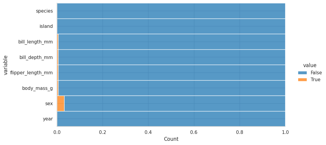
Los valores nulos no llegan ni al 10%

What are the records that contain the null values in the dataset? (Visualize)

First create the dataframe

nulls = df.isnull().transpose()
nulls

	0	1	2	3	4	5	6	7	8	9	...	334	335	336	337	338	339	340	341	342	343
species	False	False	False	False	False	False	False	False	False	False	...	False	False	False	False	False	False	False	False	False	False
island	False	False	False	False	False	False	False	False	False	False	...	False	False	False	False	False	False	False	False	False	False
bill_length_mm	False	False	False	True	False	False	False	False	False	False	...	False	False	False	False	False	False	False	False	False	False
bill_depth_mm	False	False	False	True	False	False	False	False	False	False	...	False	False	False	False	False	False	False	False	False	False
flipper_length_mm	False	False	False	True	False	False	False	False	False	False	...	False	False	False	False	False	False	False	False	False	False
body_mass_g	False	False	False	True	False	False	False	False	False	False	...	False	False	False	False	False	False	False	False	False	False
sex	False	False	False	True	False	False	False	False	True	True	...	False	False	False	False	False	False	False	False	False	False
year	False	False	False	False	False	False	False	False	False	False	...	False	False	False	False	False	False	False	False	False	False

8 rows × 344 columns

Now the chart

plt.figure(figsize=(7, 7))
nulls.pipe(
    lambda x : sns.heatmap(data=x)
)

# Alternatively, use:
#df.isnull().transpose().pipe(lambda x : sns.heatmap(data=x))

<AxesSubplot: >

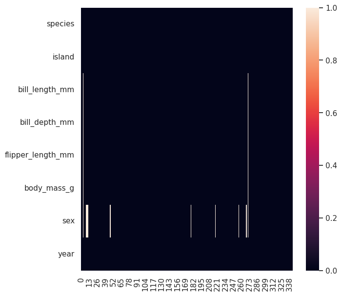
Here you can evidence:

• The missing values (Not corresponding to sex) are associated with only two records

• The sex missing values are consistant, we should not worry about that

• You might want to delete those two records that contain the vast majority of missing values (Not corresponding to sex)

How many records will be lost if we delete all the missing values?

df.dropna()

	species	island	bill_length_mm	bill_depth_mm	flipper_length_mm	body_mass_g	sex	year
0	Adelie	Torgersen	39.1	18.7	181.0	3750.0	male	2007
1	Adelie	Torgersen	39.5	17.4	186.0	3800.0	female	2007
2	Adelie	Torgersen	40.3	18.0	195.0	3250.0	female	2007
4	Adelie	Torgersen	36.7	19.3	193.0	3450.0	female	2007
5	Adelie	Torgersen	39.3	20.6	190.0	3650.0	male	2007
...	...	...	...	...	...	...	...	...
339	Chinstrap	Dream	55.8	19.8	207.0	4000.0	male	2009
340	Chinstrap	Dream	43.5	18.1	202.0	3400.0	female	2009
341	Chinstrap	Dream	49.6	18.2	193.0	3775.0	male	2009
342	Chinstrap	Dream	50.8	19.0	210.0	4100.0	male	2009
343	Chinstrap	Dream	50.2	18.7	198.0	3775.0	female	2009

333 rows × 8 columns

Note that now you have 333 rows, instead of the original 344

THIS COMMAND DOES NOT MODIFY YOUR ORIGINAL DATABASE!!!!

df.shape

(344, 8)

DO YOU SEE?

SO, LET’S SAVE IT into another variable ;)

df_clean = df.dropna()

df_clean

	species	island	bill_length_mm	bill_depth_mm	flipper_length_mm	body_mass_g	sex	year
0	Adelie	Torgersen	39.1	18.7	181.0	3750.0	male	2007
1	Adelie	Torgersen	39.5	17.4	186.0	3800.0	female	2007
2	Adelie	Torgersen	40.3	18.0	195.0	3250.0	female	2007
4	Adelie	Torgersen	36.7	19.3	193.0	3450.0	female	2007
5	Adelie	Torgersen	39.3	20.6	190.0	3650.0	male	2007
...	...	...	...	...	...	...	...	...
339	Chinstrap	Dream	55.8	19.8	207.0	4000.0	male	2009
340	Chinstrap	Dream	43.5	18.1	202.0	3400.0	female	2009
341	Chinstrap	Dream	49.6	18.2	193.0	3775.0	male	2009
342	Chinstrap	Dream	50.8	19.0	210.0	4100.0	male	2009
343	Chinstrap	Dream	50.2	18.7	198.0	3775.0	female	2009

333 rows × 8 columns

Counts and Proportions

What measures describe our dataset?

The function .describe() can do this for us, but it will just do it for numerical variables.

To include strings use .describe(include=”all”)

df.describe(include="all")

	species	island	bill_length_mm	bill_depth_mm	flipper_length_mm	body_mass_g	sex	year
count	344	344	342.000000	342.000000	342.000000	342.000000	333	344.000000
unique	3	3	NaN	NaN	NaN	NaN	2	NaN
top	Adelie	Biscoe	NaN	NaN	NaN	NaN	male	NaN
freq	152	168	NaN	NaN	NaN	NaN	168	NaN
mean	NaN	NaN	43.921930	17.151170	200.915205	4201.754386	NaN	2008.029070
std	NaN	NaN	5.459584	1.974793	14.061714	801.954536	NaN	0.818356
min	NaN	NaN	32.100000	13.100000	172.000000	2700.000000	NaN	2007.000000
25%	NaN	NaN	39.225000	15.600000	190.000000	3550.000000	NaN	2007.000000
50%	NaN	NaN	44.450000	17.300000	197.000000	4050.000000	NaN	2008.000000
75%	NaN	NaN	48.500000	18.700000	213.000000	4750.000000	NaN	2009.000000
max	NaN	NaN	59.600000	21.500000	231.000000	6300.000000	NaN	2009.000000

What if i want only numerical variables?

df.describe(include=[np.number])

	bill_length_mm	bill_depth_mm	flipper_length_mm	body_mass_g	year
count	342.000000	342.000000	342.000000	342.000000	344.000000
mean	43.921930	17.151170	200.915205	4201.754386	2008.029070
std	5.459584	1.974793	14.061714	801.954536	0.818356
min	32.100000	13.100000	172.000000	2700.000000	2007.000000
25%	39.225000	15.600000	190.000000	3550.000000	2007.000000
50%	44.450000	17.300000	197.000000	4050.000000	2008.000000
75%	48.500000	18.700000	213.000000	4750.000000	2009.000000
max	59.600000	21.500000	231.000000	6300.000000	2009.000000

What if i want only categorical variables?

df.describe(include=object)

	species	island	sex
count	344	344	333
unique	3	3	2
top	Adelie	Biscoe	male
freq	152	168	168

BONUS: Transform an object into a category

See how to transform a column with the data type “object into a category”

This allows cool things such as see the proportions

df.astype({
        "species":"category",       #just insert a dict where key is column name and value is the type
        "island":"category",
        "sex":"category"
    })

	species	island	bill_length_mm	bill_depth_mm	flipper_length_mm	body_mass_g	sex	year
0	Adelie	Torgersen	39.1	18.7	181.0	3750.0	male	2007
1	Adelie	Torgersen	39.5	17.4	186.0	3800.0	female	2007
2	Adelie	Torgersen	40.3	18.0	195.0	3250.0	female	2007
3	Adelie	Torgersen	NaN	NaN	NaN	NaN	NaN	2007
4	Adelie	Torgersen	36.7	19.3	193.0	3450.0	female	2007
...	...	...	...	...	...	...	...	...
339	Chinstrap	Dream	55.8	19.8	207.0	4000.0	male	2009
340	Chinstrap	Dream	43.5	18.1	202.0	3400.0	female	2009
341	Chinstrap	Dream	49.6	18.2	193.0	3775.0	male	2009
342	Chinstrap	Dream	50.8	19.0	210.0	4100.0	male	2009
343	Chinstrap	Dream	50.2	18.7	198.0	3775.0	female	2009

344 rows × 8 columns

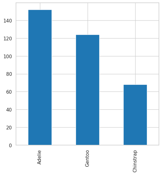
How to visualize counts?

Pandas

plt.figure(figsize=(6, 6))
df.species.value_counts().plot(kind="bar");

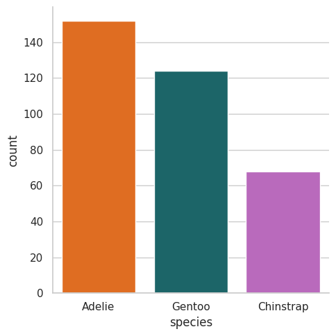
Seaborn

sns.catplot(data=df, x="species", kind="count", palette=penguin_color);

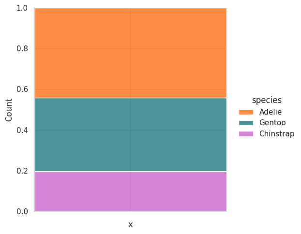
How to visualize proportions

Seaborn

df.add_column("x", "").pipe(
    lambda df: (
        sns.displot(data=df, x="x", hue="species", multiple="fill", palette=penguin_color)
    )
);

Measures of central tendency

Mean

for all the variables

df.mean()

/tmp/ipykernel_1302/3698961737.py:1: FutureWarning: The default value of numeric_only in DataFrame.mean is deprecated. In a future version, it will default to False. In addition, specifying 'numeric_only=None' is deprecated. Select only valid columns or specify the value of numeric_only to silence this warning.
  df.mean()

bill_length_mm         43.921930
bill_depth_mm          17.151170
flipper_length_mm     200.915205
body_mass_g          4201.754386
year                 2008.029070
dtype: float64

A penguin is around 4 kg LOLLLLLL

Only one variable

df.bill_depth_mm.mean()

17.151169590643274

Median

df.median()

/tmp/ipykernel_1302/530051474.py:1: FutureWarning: The default value of numeric_only in DataFrame.median is deprecated. In a future version, it will default to False. In addition, specifying 'numeric_only=None' is deprecated. Select only valid columns or specify the value of numeric_only to silence this warning.
  df.median()

bill_length_mm         44.45
bill_depth_mm          17.30
flipper_length_mm     197.00
body_mass_g          4050.00
year                 2008.00
dtype: float64

Mode

df.mode()

	species	island	bill_length_mm	bill_depth_mm	flipper_length_mm	body_mass_g	sex	year
0	Adelie	Biscoe	41.1	17.0	190.0	3800.0	male	2009

Works for categorical too

Measures of dispersion

Maximum value for each variable?

df.max(numeric_only=True)           #numeric_only=True excludes the categorical variables(makes sense)

bill_length_mm         59.6
bill_depth_mm          21.5
flipper_length_mm     231.0
body_mass_g          6300.0
year                 2009.0
dtype: float64

Minimum value for each variable?

df.min(numeric_only=True)

bill_length_mm         32.1
bill_depth_mm          13.1
flipper_length_mm     172.0
body_mass_g          2700.0
year                 2007.0
dtype: float64

Range of each variable

df.max(numeric_only=True) - df.min(numeric_only=True)

bill_length_mm         27.5
bill_depth_mm           8.4
flipper_length_mm      59.0
body_mass_g          3600.0
year                    2.0
dtype: float64

Standart deviation

df.std()

/tmp/ipykernel_1302/3390915376.py:1: FutureWarning: The default value of numeric_only in DataFrame.std is deprecated. In a future version, it will default to False. In addition, specifying 'numeric_only=None' is deprecated. Select only valid columns or specify the value of numeric_only to silence this warning.
  df.std()

bill_length_mm         5.459584
bill_depth_mm          1.974793
flipper_length_mm     14.061714
body_mass_g          801.954536
year                   0.818356
dtype: float64

Interquartile range?

The IQR equals Q3-Q1, and it holds the 50% of the data around the mean

Q1

df.quantile(0.25)

/tmp/ipykernel_1302/3656653379.py:1: FutureWarning: The default value of numeric_only in DataFrame.quantile is deprecated. In a future version, it will default to False. Select only valid columns or specify the value of numeric_only to silence this warning.
  df.quantile(0.25)

bill_length_mm         39.225
bill_depth_mm          15.600
flipper_length_mm     190.000
body_mass_g          3550.000
year                 2007.000
Name: 0.25, dtype: float64

Q3

df.quantile(0.75)

/tmp/ipykernel_1302/3799946287.py:1: FutureWarning: The default value of numeric_only in DataFrame.quantile is deprecated. In a future version, it will default to False. Select only valid columns or specify the value of numeric_only to silence this warning.
  df.quantile(0.75)

bill_length_mm         48.5
bill_depth_mm          18.7
flipper_length_mm     213.0
body_mass_g          4750.0
year                 2009.0
Name: 0.75, dtype: float64

IQR

(
    df
    .quantile(q=[0.75, 0.50, 0.25])
    .transpose()
    .rename_axis("variable")
    .reset_index()
    .assign(
        iqr=lambda df: df[0.75] - df[0.25]
    )
)

/tmp/ipykernel_1302/4097684495.py:2: FutureWarning: The default value of numeric_only in DataFrame.quantile is deprecated. In a future version, it will default to False. Select only valid columns or specify the value of numeric_only to silence this warning.
  df

	variable	0.75	0.5	0.25	iqr
0	bill_length_mm	48.5	44.45	39.225	9.275
1	bill_depth_mm	18.7	17.30	15.600	3.100
2	flipper_length_mm	213.0	197.00	190.000	23.000
3	body_mass_g	4750.0	4050.00	3550.000	1200.000
4	year	2009.0	2008.00	2007.000	2.000

Probabilities

Probability Mass function

Probability for each value

empiricaldist.Pmf.from_seq(df.flipper_length_mm)

	probs
172.0	0.002924
174.0	0.002924
176.0	0.002924
178.0	0.011696
179.0	0.002924
180.0	0.014620
181.0	0.020468
182.0	0.008772
183.0	0.005848
184.0	0.020468
185.0	0.026316
186.0	0.020468
187.0	0.046784
188.0	0.017544
189.0	0.020468
190.0	0.064327
191.0	0.038012
192.0	0.020468
193.0	0.043860
194.0	0.014620
195.0	0.049708
196.0	0.029240
197.0	0.029240
198.0	0.023392
199.0	0.017544
200.0	0.011696
201.0	0.017544
202.0	0.011696
203.0	0.014620
205.0	0.008772
206.0	0.002924
207.0	0.005848
208.0	0.023392
209.0	0.014620
210.0	0.040936
211.0	0.005848
212.0	0.020468
213.0	0.017544
214.0	0.017544
215.0	0.035088
216.0	0.023392
217.0	0.017544
218.0	0.014620
219.0	0.014620
220.0	0.023392
221.0	0.014620
222.0	0.017544
223.0	0.005848
224.0	0.008772
225.0	0.011696
226.0	0.002924
228.0	0.011696
229.0	0.005848
230.0	0.020468
231.0	0.002924

Then, if i want to know that is the specific probability of getting a value:

empiricaldist.Pmf.from_seq(df.flipper_length_mm)(190)

0.06432748538011696

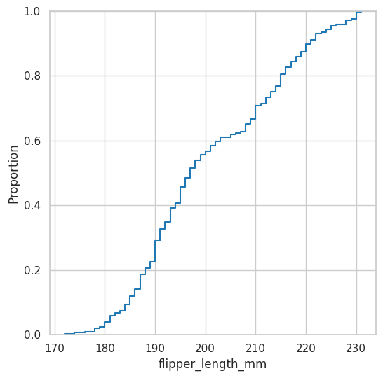
Empirical Cumulative Distribution Function

This one returns the cumulative probability based on the dataset

plt.figure(figsize=(6, 6))
sns.ecdfplot(data=df, x="flipper_length_mm");

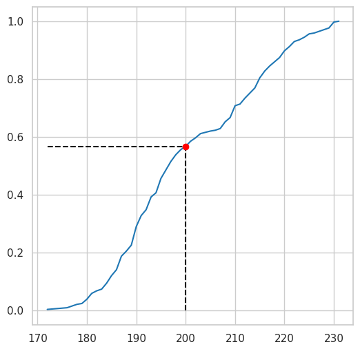
Probabilities of getting a penguin with 200 or less flipper_length?

empiricaldist.Cdf.from_seq(df.flipper_length_mm)(200)

array(0.56725146)

See the chart below for a better interpretation

plt.figure(figsize=(6, 6))

empiricaldist.Cdf.from_seq(df.flipper_length_mm).plot()

q=200
p = empiricaldist.Cdf.from_seq(df.flipper_length_mm)(200)

plt.vlines(
    x=q,
    ymin=0,
    ymax=p,
    color="black",
    linestyle="dashed"
)

plt.hlines(
    y=p,
    xmin=empiricaldist.Cdf.from_seq(df.flipper_length_mm).qs[0],
    xmax=q,
    color="black",
    linestyle="dashed"
)

plt.plot(q, p, "ro");

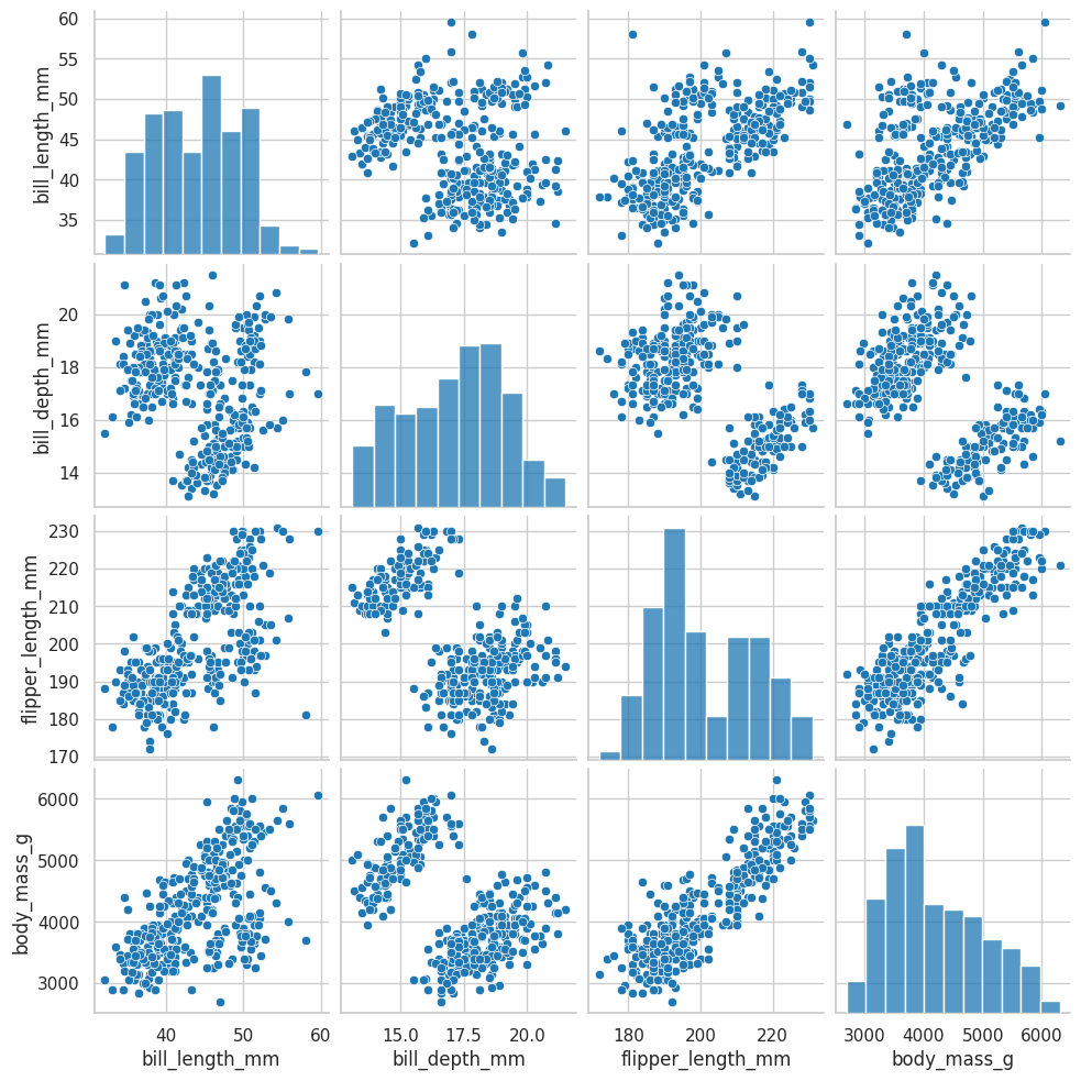
Correlations

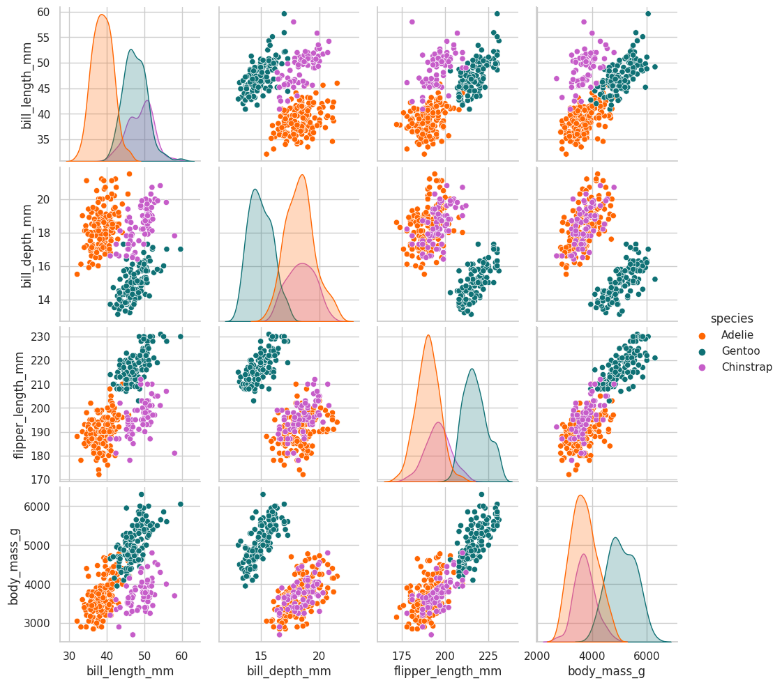
Pairplot

In this case, please remove the year column, despite being a numeric column, it is not adding value to the correlation analysis

sns.pairplot(data=df.drop(["year"], axis=1));

Pairplot per specie

sns.pairplot(data=df.drop(["year"], axis=1), hue="species", palette=penguin_color);

Swarmplot

This one can be used to associate a categorical variable with a numerical:

plt.figure(figsize=(6, 6))
sns.swarmplot(
    data=df,
    x="island",
    y="body_mass_g",
    hue="species",
    palette=penguin_color
);

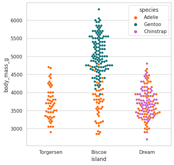
• There doesn’t seem to be a relation among the penguin body mass and the island where it is located

• there is a relation among the body mass and the specie

Is there a linear correlation among any of our variables?

df.drop(["year"], axis=1).corr()          #first remove the year column and then run

/tmp/ipykernel_1302/2116061803.py:1: FutureWarning: The default value of numeric_only in DataFrame.corr is deprecated. In a future version, it will default to False. Select only valid columns or specify the value of numeric_only to silence this warning.
  df.drop(["year"], axis=1).corr()          #first remove the year column and then run

	bill_length_mm	bill_depth_mm	flipper_length_mm	body_mass_g
bill_length_mm	1.000000	-0.235053	0.656181	0.595110
bill_depth_mm	-0.235053	1.000000	-0.583851	-0.471916
flipper_length_mm	0.656181	-0.583851	1.000000	0.871202
body_mass_g	0.595110	-0.471916	0.871202	1.000000

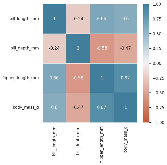
• Flipper length and body mass have a 0.8712 correlation coef, high

let’s visualize that into a matrix

plt.figure(figsize=(6, 6))
sns.heatmap(
    data=df.drop(["year"], axis=1).corr(),
    cmap=sns.diverging_palette(20, 230, as_cmap=True),        #nice color palette
    center=0,                                                 #centering the color legend
    vmin=-1,                                                  #set min corr value to -1
    vmax=1,                                                   #set max corr value to 1
    linewidths=0.5,
    annot=True
)

/tmp/ipykernel_1302/2892716928.py:3: FutureWarning: The default value of numeric_only in DataFrame.corr is deprecated. In a future version, it will default to False. Select only valid columns or specify the value of numeric_only to silence this warning.
  data=df.drop(["year"], axis=1).corr(),

<AxesSubplot: >

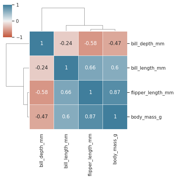
sns.clustermap(
    data=df.drop(["year"], axis=1).corr(),
    cmap=sns.diverging_palette(20, 230, as_cmap=True),        #nice color palette
    center=0,                                                 #centering the color legend
    vmin=-1,                                                  #set min corr value to -1
    vmax=1,                                                   #set max corr value to 1
    linewidths=0.5,
    annot=True,
    figsize=(6,6)
);

/tmp/ipykernel_1302/2652653307.py:2: FutureWarning: The default value of numeric_only in DataFrame.corr is deprecated. In a future version, it will default to False. Select only valid columns or specify the value of numeric_only to silence this warning.
  data=df.drop(["year"], axis=1).corr(),

How can i represent a categorical variable as a discrete numerical?

Let’s do it with sex, set female to 0 and male to 1

df = df.assign(
    numeric_sex=lambda df : df.sex.replace(["female", "male"], [0, 1])
)

df_clean = df.dropna()

sns.clustermap(
    data=df.drop(["year"], axis=1).corr(),
    cmap=sns.diverging_palette(20, 230, as_cmap=True),        #nice color palette
    center=0,                                                 #centering the color legend
    vmin=-1,                                                  #set min corr value to -1
    vmax=1,                                                   #set max corr value to 1
    linewidths=0.5,
    annot=True,
    figsize=(6,6)
);

/tmp/ipykernel_1302/2652653307.py:2: FutureWarning: The default value of numeric_only in DataFrame.corr is deprecated. In a future version, it will default to False. Select only valid columns or specify the value of numeric_only to silence this warning.
  data=df.drop(["year"], axis=1).corr(),

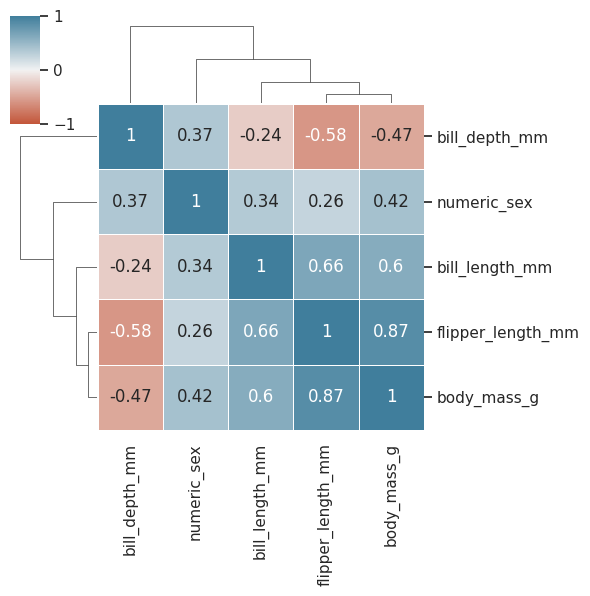
Look like linear correlation is low among sex and the other variables

Multiple regression

I forgot the scale to weigh the penguins, what is the best way to capture that data?

Let’s create many linear regression models and compare them

• Use the df_clean, which contains the dataset without null values, just to avoid errors

Model 1

let’s create a model to predict the “body_mass” using the variable “bill_depth”

#Creating the model

model_1 = (
    smf.ols(
        formula="body_mass_g ~ bill_length_mm",
        data=df_clean
    )
    .fit()
)

#Describing the model

model_1.summary()

OLS Regression Results

Dep. Variable:	body_mass_g	R-squared:	0.347
Model:	OLS	Adj. R-squared:	0.345
Method:	Least Squares	F-statistic:	176.2
Date:	Mon, 09 Jan 2023	Prob (F-statistic):	1.54e-32
Time:	21:34:02	Log-Likelihood:	-2629.1
No. Observations:	333	AIC:	5262.
Df Residuals:	331	BIC:	5270.
Df Model:	1
Covariance Type:	nonrobust

	coef	std err	t	P>|t|	[0.025	0.975]
Intercept	388.8452	289.817	1.342	0.181	-181.271	958.961
bill_length_mm	86.7918	6.538	13.276	0.000	73.931	99.652

Omnibus:	6.141	Durbin-Watson:	0.849
Prob(Omnibus):	0.046	Jarque-Bera (JB):	4.899
Skew:	-0.197	Prob(JB):	0.0864
Kurtosis:	2.555	Cond. No.	360.

Notes:
[1] Standard Errors assume that the covariance matrix of the errors is correctly specified.

Model 2

Now let’s add a second variable “bill_depth_mm”

#Creating the model

model_2 = (
    smf.ols(
        formula="body_mass_g ~ bill_length_mm + bill_depth_mm",
        data=df_clean
    )
    .fit()
)

#Describing the model

model_2.summary()

OLS Regression Results

Dep. Variable:	body_mass_g	R-squared:	0.467
Model:	OLS	Adj. R-squared:	0.464
Method:	Least Squares	F-statistic:	144.8
Date:	Mon, 09 Jan 2023	Prob (F-statistic):	7.04e-46
Time:	21:34:02	Log-Likelihood:	-2595.2
No. Observations:	333	AIC:	5196.
Df Residuals:	330	BIC:	5208.
Df Model:	2
Covariance Type:	nonrobust

	coef	std err	t	P>|t|	[0.025	0.975]
Intercept	3413.4519	437.911	7.795	0.000	2552.002	4274.902
bill_length_mm	74.8126	6.076	12.313	0.000	62.860	86.765
bill_depth_mm	-145.5072	16.873	-8.624	0.000	-178.699	-112.315

Omnibus:	2.839	Durbin-Watson:	1.798
Prob(Omnibus):	0.242	Jarque-Bera (JB):	2.175
Skew:	-0.000	Prob(JB):	0.337
Kurtosis:	2.604	Cond. No.	644.

Notes:
[1] Standard Errors assume that the covariance matrix of the errors is correctly specified.

Model 3

Now we can add the “flipper_length_mm” and see what happens

#Creating the model

model_3 = (
    smf.ols(
        formula="body_mass_g ~ bill_length_mm + bill_depth_mm + flipper_length_mm",
        data=df_clean
    )
    .fit()
)

#Describing the model

model_3.summary()

OLS Regression Results

Dep. Variable:	body_mass_g	R-squared:	0.764
Model:	OLS	Adj. R-squared:	0.762
Method:	Least Squares	F-statistic:	354.9
Date:	Mon, 09 Jan 2023	Prob (F-statistic):	9.26e-103
Time:	21:34:02	Log-Likelihood:	-2459.8
No. Observations:	333	AIC:	4928.
Df Residuals:	329	BIC:	4943.
Df Model:	3
Covariance Type:	nonrobust

	coef	std err	t	P>|t|	[0.025	0.975]
Intercept	-6445.4760	566.130	-11.385	0.000	-7559.167	-5331.785
bill_length_mm	3.2929	5.366	0.614	0.540	-7.263	13.849
bill_depth_mm	17.8364	13.826	1.290	0.198	-9.362	45.035
flipper_length_mm	50.7621	2.497	20.327	0.000	45.850	55.675

Omnibus:	5.596	Durbin-Watson:	1.982
Prob(Omnibus):	0.061	Jarque-Bera (JB):	5.469
Skew:	0.312	Prob(JB):	0.0649
Kurtosis:	3.068	Cond. No.	5.44e+03

Notes:
[1] Standard Errors assume that the covariance matrix of the errors is correctly specified.
[2] The condition number is large, 5.44e+03. This might indicate that there are
strong multicollinearity or other numerical problems.

Model 4

#Creating the model

model_4 = (
    smf.ols(
        formula="body_mass_g ~ bill_length_mm + bill_depth_mm + flipper_length_mm + C(sex)",
        data=df_clean
    )
    .fit()
)

#Describing the model

model_4.summary()

OLS Regression Results

Dep. Variable:	body_mass_g	R-squared:	0.823
Model:	OLS	Adj. R-squared:	0.821
Method:	Least Squares	F-statistic:	381.3
Date:	Mon, 09 Jan 2023	Prob (F-statistic):	6.28e-122
Time:	21:34:02	Log-Likelihood:	-2411.8
No. Observations:	333	AIC:	4834.
Df Residuals:	328	BIC:	4853.
Df Model:	4
Covariance Type:	nonrobust

	coef	std err	t	P>|t|	[0.025	0.975]
Intercept	-2288.4650	631.580	-3.623	0.000	-3530.924	-1046.006
C(sex)[T.male]	541.0285	51.710	10.463	0.000	439.304	642.753
bill_length_mm	-2.3287	4.684	-0.497	0.619	-11.544	6.886
bill_depth_mm	-86.0882	15.570	-5.529	0.000	-116.718	-55.459
flipper_length_mm	38.8258	2.448	15.862	0.000	34.011	43.641

Omnibus:	2.598	Durbin-Watson:	1.843
Prob(Omnibus):	0.273	Jarque-Bera (JB):	2.125
Skew:	0.062	Prob(JB):	0.346
Kurtosis:	2.629	Cond. No.	7.01e+03

Notes:
[1] Standard Errors assume that the covariance matrix of the errors is correctly specified.
[2] The condition number is large, 7.01e+03. This might indicate that there are
strong multicollinearity or other numerical problems.

Model 5

Let’s now try with the “flipper_length_mm” alone

#Creating the model

model_5 = (
    smf.ols(
        formula="body_mass_g ~ flipper_length_mm + C(sex)",
        data=df_clean
    )
    .fit()
)

#Describing the model

model_5.summary()

OLS Regression Results

Dep. Variable:	body_mass_g	R-squared:	0.806
Model:	OLS	Adj. R-squared:	0.805
Method:	Least Squares	F-statistic:	684.8
Date:	Mon, 09 Jan 2023	Prob (F-statistic):	3.53e-118
Time:	21:34:02	Log-Likelihood:	-2427.2
No. Observations:	333	AIC:	4860.
Df Residuals:	330	BIC:	4872.
Df Model:	2
Covariance Type:	nonrobust

	coef	std err	t	P>|t|	[0.025	0.975]
Intercept	-5410.3002	285.798	-18.931	0.000	-5972.515	-4848.085
C(sex)[T.male]	347.8503	40.342	8.623	0.000	268.491	427.209
flipper_length_mm	46.9822	1.441	32.598	0.000	44.147	49.817

Omnibus:	0.262	Durbin-Watson:	1.710
Prob(Omnibus):	0.877	Jarque-Bera (JB):	0.376
Skew:	0.051	Prob(JB):	0.829
Kurtosis:	2.870	Cond. No.	2.95e+03

Notes:
[1] Standard Errors assume that the covariance matrix of the errors is correctly specified.
[2] The condition number is large, 2.95e+03. This might indicate that there are
strong multicollinearity or other numerical problems.

Note that only one variable explains the 76% of the variance.

You decide if sticking with one variable and getting 76% of variance, or stick with 4 and get 80%.

Multiple Regression Model Comparisons

Creation of a results table

model_results = pd.DataFrame(
    dict(
        actual_value = df_clean.body_mass_g,
        prediction_model_1 = model_1.predict(),
        prediction_model_2 = model_2.predict(),
        prediction_model_3 = model_3.predict(),
        prediction_model_4 = model_4.predict(),
        prediction_model_5 = model_5.predict(),
        species = df_clean.species,
        sex = df_clean.sex
    )
)

model_results

	actual_value	prediction_model_1	prediction_model_2	prediction_model_3	prediction_model_4	prediction_model_5	species	sex
0	3750.0	3782.402961	3617.641192	3204.761227	3579.136946	3441.323750	Adelie	male
1	3800.0	3817.119665	3836.725580	3436.701722	3343.220772	3328.384372	Adelie	female
2	3250.0	3886.553073	3809.271371	3906.897032	3639.137335	3751.223949	Adelie	female
4	3450.0	3574.102738	3350.786581	3816.705772	3457.954243	3657.259599	Adelie	female
5	3650.0	3799.761313	3356.140070	3696.168128	3764.536023	3864.163327	Adelie	male
...	...	...	...	...	...	...	...	...
339	4000.0	5231.825347	4706.954140	4599.187485	4455.022405	4662.860306	Chinstrap	male
340	3400.0	4164.286703	4034.121055	4274.552753	3894.857519	4080.099176	Chinstrap	female
341	3775.0	4693.716437	4475.927353	3839.563668	4063.639819	4005.109853	Chinstrap	male
342	4100.0	4797.866549	4449.296758	4720.740455	4652.013882	4803.806832	Chinstrap	male
343	3775.0	4745.791493	4448.061337	4104.268240	3672.299099	3892.170475	Chinstrap	female

333 rows × 8 columns

Comparing predicted values vs Actual values (ECDFs)

plt.figure(figsize=(6, 6))
sns.ecdfplot(
    data=model_results
);

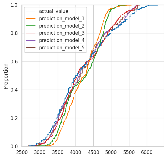
Now, note that the BLUE LINE ARE THE ACTUAL VALUES

Therefore, the line that is closer to the model, would be the better model

Comparing predicted values distributions vs Original values distributions(Kdeplot)

plt.figure(figsize=(6, 6))
sns.kdeplot(
    data=model_results
);

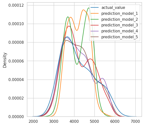
Looks like the purple line (model 4) fits better, but that contains 4 variables.

The model 5 also fist really great with only two variables

Bonus: Pandas Profiling Report

import palmerpenguins
import pandas as pd
import pandas_profiling as pp

df = palmerpenguins.load_penguins()

pp.ProfileReport(df)

Created in Deepnote